4.42 Execution profiling
This section describes the hierarchical execution profiler. This
profiler is based on ideas from gprof described in
Graham et
al., 1982. The profiler consists of two parts: the
information-gathering component built into the kernel,165There
are two implementations; one based on setitimer() using the SIGPROF
signal and one using Windows Multi Media (MM) timers. On other systems
the profiler is not provided. and a presentation component
which is defined in the library(statistics) library. The
latter can be hooked, which is used by the XPCE module
library(swi/pce_profile) to provide an interactive
graphical frontend for the results.
4.42.1 library(prolog_profile): Execution profiler
This module provides a simple frontend on the execution profiler with
a hook to the GUI visualiser for profiling results defined in
library(swi/pce_profile).
- profile(:Goal)
- profile(:Goal, +Options)
- Run
once(Goal)under the execution profiler. If the (xpce) GUI is enabled this predicate is hooked bylibrary(swi/pce_profile)and results are presented in a gui that enables navigating the call tree and jump to predicate implementations. Without the GUI, a simple textual report is generated. Defined options are:- time(Which)
- Profile
cpuorwalltime. The default is CPU time. - exact(Exact)
- If
true, do not sample, but read the clock each time execution moves to another node of the call tree. This gives exact wall times, also for short running goals. For CPU time, the thread's CPU time is read once per sample period (seesample_rate(Rate)) and after each long interval, where the thread may have been off the CPU. Ifauto, use exact timing if reading the clock is cheap and, for CPU time, the thread CPU clock is precise. This is typically not the case in virtual machines. Otherwise use sampling. Default is defined by the Prolog flag profile_exact, which defaults toauto. - sample_rate(Rate)
- Samples per second, any numeric value between 1 and 1000. Default is defined by the Prolog flag profile_sample_rate, which defaults to 200.
- ports(Bool)
- Specifies ports counted -
true(all ports),false(call port only) orclassic(all with some errors). Accomodates space/accuracy tradeoff building call tree. Default is defined by the Prolog flag profile_ports, which defaults totrue. - top(N)
- When generating a textual report, show the top N predicates.
- cumulative(Bool)
- If
true(defaultfalse), show cumulative output in a textual report. - measure(Measure)
- When generating a textual report, show
time(default) ormemory, the global stack allocated and discarded by backtracking. See show_profile/1.
- show_profile(+Options)
- Display last collected profiling data. Options are
- top(N)
- When generating a textual report, show the top N predicates.
- cumulative(Bool)
- If
true(defaultfalse), show cumulative output in a textual report. - measure(Measure)
- One of
time(default) ormemory. The latter shows the global stack allocated by the predicate itself and by its callees, and the global stack discarded by backtracking into the predicate. For example, forp :- \+ \+ q, q allocates and p discards. The predicates are sorted on the allocated memory.
- [det]profile_data(-Data)
- Gather all relevant data from profiler. This predicate may be called
while profiling is active in which case it is suspended while collecting
the data. Data is a dict providing the following fields:
summary:Dict- Overall statistics providing
- samples:Count: Times the statistical profiler was called or, if
exactistrue, the number of times execution moved to another node of the call tree. - ticks:Count Nanoseconds sampled during profiling
- accounting:Count Nanoseconds spent on accounting. This is the profiler's own overhead. The exact modes measure it and exclude it from the times of the predicates.
- time:Seconds Total time sampled
- nodes:Count Nodes in the call graph.
- sample_period: MicroSeconds Same interval timer period in micro seconds
- ports: Ports One of
true,falseorclassic - clock: Clock One of
cpuorwall, the time that was profiled. - exact: Bool Whether the data was collected using
exact(true) - allocated: Bytes
- discarded: Bytes
- gc_reclaimed: Bytes Global stack allocated, discarded by backtracking and reclaimed by garbage collection while profiling.
- gc_count: Count Number of garbage collections while profiling.
- samples:Count: Times the statistical profiler was called or, if
- nodes
- List of nodes. Each node provides:
predicate:PredicateIndicator- or a blob that represents another profiled object, such as an XPCE method.
ticks_self:Countticks_siblings:Count- Nanoseconds sampled in the predicate itself and in its callees.
alloc_self:Bytesalloc_siblings:Bytes- Global stack allocated by the predicate itself and by its callees.
discarded_self:Bytesdiscarded_siblings:Bytes- Global stack discarded by backtracking into a choicepoint of the predicate itself and of its callees.
call:Countredo:Countexit:Countcallers:list_of(Relative)callees:list_of(Relative)
Relative is a term of the shape below that represents a caller or callee. Future versions are likely to use a dict instead.
node(PredicateIndicator, CycleID, Ticks, TicksSiblings,
     Calls, Redos, Exits, Memory)
Memory is a term
mem(Alloc, AllocSiblings, Discarded, DiscardedSiblings), the global stack in bytes allocated and discarded by these calls, by the called predicate itself and by its callees, as the ‘alloc_*anddiscarded_*` keys of the node. - [nondet]profile_procedure_data(?Pred, -Data:dict)
- Collect data for Pred. If Pred is unbound data for
each predicate that has profile data available is returned. Data
is described in
profile_data/1 as
an element of the
nodeskey.
4.42.2 Visualizing profiling data
Browsing the annotated call-tree as described in section 4.42.3 itself is not very attractive. Therefore, the results are combined per predicate, collecting all callers and callees as well as the propagation of time and activations in both directions. Figure 4 illustrates this. The central yellowish line is the ‘current’ predicate with counts for time spent in the predicate (`Self’), time spent in its children (`Siblings’), activations through the call and redo ports. Above that are the callers. Here, the two time fields indicate how much time is spent serving each of the callers. The columns sum to the time in the yellowish line. The caller <recursive> is the number of recursive calls. Below the yellowish lines are the callees, with the time spent in the callee itself for serving the current predicate and the time spent in the callees of the callee ('Siblings’), so the whole time-block adds up to the ‘Siblings’ field of the current predicate. The ‘Access’ fields show how many times the current predicate accesses each of the callees.
The predicates have a menu that allows changing the view of the detail window to the given caller or callee, showing the documentation (if it is a built-in) and/or jumping to the source.
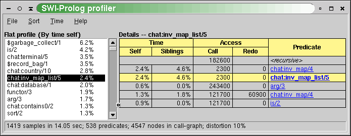
The statistics shown in the report field of figure 4 show the following information:
- samples
Number of times the call-tree was sampled for collecting time statistics. On most hardware, the resolution ofSIGPROFis 1/100 second. This number must be sufficiently large to get reliable timing figures. The Time menu allows viewing time as samples, relative time or absolute time. - sec
Total user CPU time with the profiler active. - predicates
Total count of predicates that have been called at least one time during the profile. - nodes
Number of nodes in the call-tree. - distortion
How much of the time is spent building the call-tree as a percentage of the total execution time. Timing samples while the profiler is building the call-tree are not added to the call-tree.
4.42.3 Information gathering
While the program executes under the profiler, the system builds a dynamic call-tree. It does this using three hooks from the kernel: one that starts a new goal (profCall), one that tells the system which goal is resumed after an exit (profExit) and one that tells the system which goal is resumed after a fail (i.e., which goal is used to retry (profRedo)). The profCall() function finds or creates the subnode for the argument predicate below the current node, increments the call-count of this link and returns the sub-node which is recorded in the Prolog stack-frame. Choice-points are marked with the current profiling node. profExit() and profRedo() pass the profiling node where execution resumes.
Just using the above algorithm would create a much too big tree due to recursion. For this reason the system performs detection of recursion. In the simplest case, recursive procedures increment the ‘recursive’ count on the current node. Mutual recursion, however, is not easily detected. For example, call/1 can call a predicate that uses call/1 itself. This can be viewed as a recursive invocation, but this is generally not desirable. Recursion is currently assumed if the same predicate with the same parent appears higher in the call-graph. Early experience with some non-trivial programs are promising.
The last part of the profiler collects statistics on the CPU time
used in each node. On systems providing setitimer() with
SIGPROF, it ‘ticks’ the current node of the
call-tree each time the timer fires, adding the CPU (or wall) time
elapsed since the previous tick in nanoseconds. On Windows, a MM-timer
in a separate thread checks 100 times per second how much time is spent
in the profiled thread and adds this to the current node. See section
4.42.3.1 for details.
Using the option exact(true), profile/2
does not sample, but reads a clock each time execution moves to another
node of the call tree and adds the elapsed wall time to the node that
was left. The time spent updating the call tree is reported as
accounting time. This gives exact timings, also for short running goals
and predicates that are called often but run briefly. It uses the
processor's timestamp counter if this is available (the invariant TSC on
x86 or the virtual counter on ARM64) and the operating system's
monotonic clock otherwise.
Reading the CPU time of a thread is too slow to do at every node switch. For CPU time, the exact mode therefore reads the thread's CPU time once per sample period, as well as after each interval longer than 10 microseconds. A thread can only spend significant time off the CPU, e.g., blocked in I/O or sleep/1, inside a single long interval. The short intervals are considered to have run on the CPU and the long interval is charged the remaining CPU time used in the period.
By default (Prolog flag profile_exact is auto),
profile/2
uses exact timing if reading the clock is cheap and, for CPU time, the
thread CPU time can be read precisely. This is typically not the case in
virtual machines, where reading the timestamp counter may trap into the
hypervisor. In that case profile/2
uses sampling.
4.42.3.1 Profiling in the Windows Implementation
Profiling in the Windows version is similar, but as profiling is a statistical process it is good to be aware of the implementation166We hereby acknowledge Lionel Fourquaux, who suggested the design described here after a newsnet enquiry. for proper interpretation of the results.
Windows does not provide timers that fire asynchronously, frequent and proportional to the CPU time used by the process. Windows does provide multi-media timers that can run at high frequency. Such timers, however, run in a separate thread of execution and they are fired on the wall clock rather than the amount of CPU time used. The profiler installs such a timer running, for saving CPU time, rather inaccurately at about 100 Hz. Each time it is fired, it determines the CPU time in milliseconds used by Prolog since the last time it was fired. If this value is non-zero, active predicates are incremented with this value.